The experimental setup is as follows. I use the same training data for each run, and evaluate the results on the same test set. I’m going to compare the F1 score for plants between different runs. I set up a number of runs with SGD as the solver and sweeping through momentum values from 0–0.99 (when using momentum, anything greater than 1.0 causes the solver to diverge). I set up 10 runs with momentum values from 0 to 0.9 in increments of 0.1.
Following that I performed another set of 10 runs, this time with momentum values between 0.90 and 0.99, with increments of 1. After looking at these results, I also ran a set of experiments at momentum values of 0.999 and 0.9999. Each run was done with a different random seed, and was given a tag of “SGD Sweep” in W&B. The results are shown in Figure 1.

Figure 1: On the left hand side the f1 score for crops is shown on the x-axis, and the run name is shown on the y axis. On the right hand side the f1 score for plants as a function of momentum value is shown. | Credit: Blue River Technology
It is very clear from Figure 1 that larger values of momentum are increasing the f1 score. The best value of 0.9447 occurs at momentum value of 0.999, and drops off to a value of 0.9394 at a momentum value of 0.9999. The values are shown in the table below.

Table 1: Each run is shown as a row in the table above. The last column is the momentum setting for the run. The F1 score, precision, and recall for class 2 (crops) is shown. | Credit: Blue River Technology
How do these results compare to Adam? To test this I ran 10 identical runs using torch.optim.Adam with just the default parameters. I used the tag “Adam runs” in W&B to identify these runs. I also tagged each set of SGD runs for comparison. Since a different random seed is used for each run, the solver will initialize differently each time and will end up with different weights at the last epoch. This gives slightly different results on the test set for each run. To compare them I will need to measure the spread of values for the Adam and SGD runs. This is easy to do with a box plot grouped by tag in W&B.

Figure 2: The spread of values for Adam and SGD. The Adam runs are shown in the left of the graph in green. The SGD runs are shown as brown (0.999), teal (0–0.99), blue (0.9999) and yellow (0.95). | Credit: Blue River Technology
The results are shown in graph form in Figure 2, and in tabular form in Table 2. The full report is available online too. You can see that I haven’t been able to beat the results for Adam by just adjusting momentum values with SGD. The momentum setting of 0.999 gives very comparable results, but the variance on the Adam runs is tighter and the average value is higher as well. So Adam appears to be a good choice of solver for our plant segmentation problem!
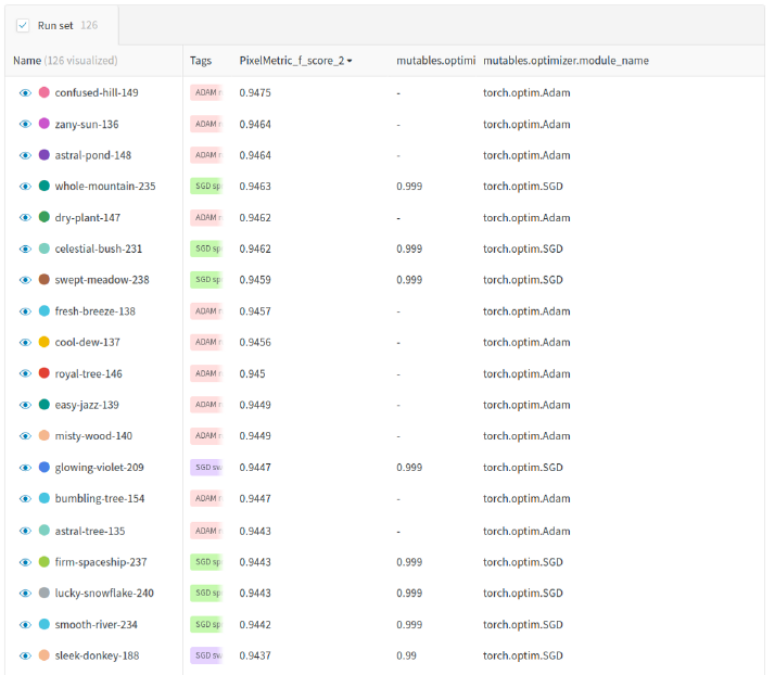
Table 2: Run table showing f1 score, optimizer and momentum value for each run. | Credit: Blue River Technology
PyTorch Visualizations
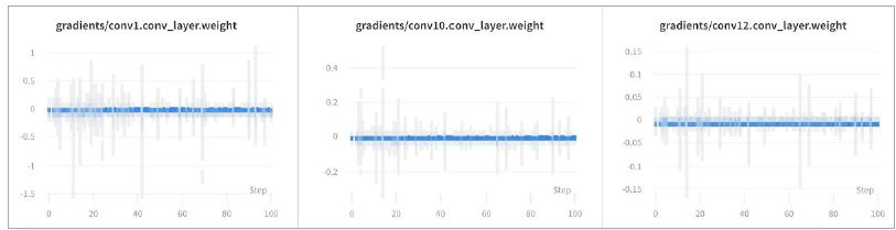
With the PyTorch integration, W&B picks up the gradients at each layer, letting us inspect the network during training.
W&B experiment tracking also makes it easy to visualize PyTorch models during training, so you can see the loss curves in real time in a central dashboard. We use these visualizations in our team meetings to discuss the latest results and share updates.
As the images pass through our PyTorch model, we seamlessly log predictions to Weights & Biases to visualize the results of model training. Here we can see the predictions, ground truth, and labels. This makes it easy to identify scenarios where model performance isn’t meeting our expectations.
Here we can quickly browse the ground truth, predictions and the difference between the two. We’ve labeled the crops in green and the weeds in red. As you can see, the model is doing a pretty reasonable job of identifying the crops and the weeds in the image.

Reproducible models
Reproducibility and traceability are key features of any ML system, and it’s hard to get right. When comparing different network architectures and hyperparameters, the input data needs to be the same to make runs comparable. Often individual practitioners on ML teams save YAML or JSON config files – it’s excruciating to find a team member’s run and wade through their config file to find out what training set and hyperparameters were used. We’ve all done it, and we all hate it.
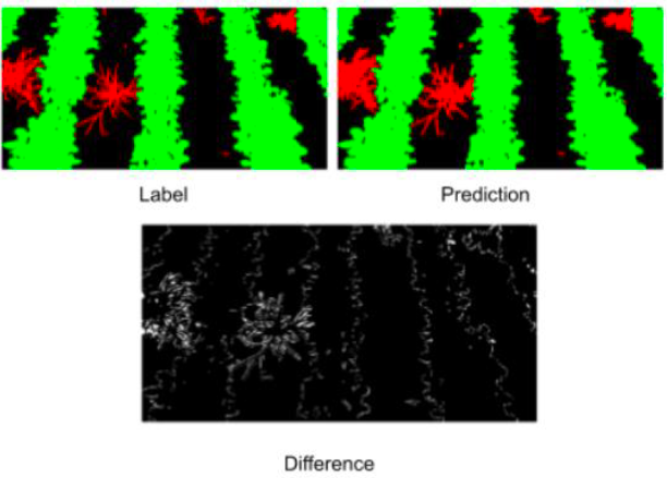
The ground truth, predictions and the difference between the two. Crops are shown in green, while weeds are shown in red. | Blue River Technology
A new feature that W&B just released solves this problem. Artifacts allow us to track the inputs and outputs of our training and evaluation runs. This helps us a lot with reproducibility and traceability. By inspecting the Artifacts section of a run in W&B I can tell what datasets were used to train the model, what models were produced (from multiple runs), and the results of the model evaluation.
A typical use case is the following. A data staging process downloads the latest and greatest data and stages it to disk for training and test (separate data sets for each). These datasets are specified as artifacts. A training run takes the training set artifact as input and outputs a trained model as an output artifact. The evaluation process takes the test set artifact as input, along with the trained model artifact, and outputs an evaluation that might include a set of metrics or images. A directed acyclic graph (DAG) is formed and visualized within W&B. This is helpful since it is very important to track the artifacts that are involved with releasing a machine learning model into production. A DAG like this can be formed easily:

Credit: Blue River Technology
One of the big advantages of the Artifacts feature is that you can choose to upload all the artifacts (datasets, models, evaluations) or you can choose to upload only references to the artifacts. This is a nice feature because moving lots of data around is time consuming and slow. With the dataset artifacts, we simply store a reference to those artifacts in W&B. That allows us to maintain control of our data (and avoid long transfer times) and still get traceability and reproducibility in machine learning.
Leading ML teams
Looking back on the years I’ve spent leading teams of machine learning engineers, I’ve seen some common challenges:
- Efficiency: As we develop new models, we need to experiment quickly and share results. PyTorch makes it easy for us to add new features fast, and Weights & Biases gives us the visibility we need to debug and improve our models.
- Flexibility: Working with our customers in the fields, every day can bring a new challenge. Our team needs tools that can keep up with our constantly evolving needs, which is why we chose PyTorch for its thriving ecosystem and W&B for the lightweight, modular integrations.
- Performance: At the end of the day, we need to build the most accurate and fastest models for our field machines. PyTorch enables us to iterate quickly, then productionize our models and deploy them in the field. We have full visibility and transparency in the development process with W&B, making it easy to identify the most performant models.
I hope you have enjoyed this short tour of how my team uses PyTorch and Weights and Biases to enable the next generation of intelligent agricultural machines!
About the Author
Chris Padwick is the director of computer vision and machine learning at Blue River Technology. The company was acquired by John Deere in 2017 for $305 million.


Tell Us What You Think!